Feature Story

Maintenance Station Location Model

By Gene Hewitt and Amie Drotning

One of the fundamental questions that we have in public works is where to locate maintenance yards to best serve the public and maintain infrastructure assets — roads, stormwater, sewer, water, etc. The location(s) can affect the service, cost, response time, and ability to maintain assets. One way to evaluate maintenance yard locations is through the use of a Maintenance Station Location Model (MSLM).

The information generated by an MSLM can provide the framework for determining whether to add new maintenance stations or yards; or to relocate, consolidate, renovate, close, or adjust staff levels among existing yards.

This article discusses the use of a model (MSLM) to quantify maintenance travel, operations, and capital costs. The model can be used to generate justification for decisions on maintenance yard locations through properly documenting the process. This discusses the theory as well as a specific example of how this was applied in Santa Clara, Calif., to determine the best location for these yards.

Background

Santa Clara County Roads and Airports Department (RAD) maintains a road network of approximately 705 centerline miles and covers an area of 1,290 square miles. The county population is approximately 1.8 million and has grown 5.9 percent from 2000 to 2010. The population is expected to continue growing approximately 6.9 percent annually to 2016. Three maintenance yards for the department exist throughout Santa Clara County (West, East, and South) with varying staffing levels and work environments. The West and East yards serve primarily urban areas with the South yard located in the rural area of the county.

The department sought to analyze the need for its existing maintenance yards while estimating the impact of a number of alternative yard configurations. RAD management recognized that the following factors demonstrated the importance of undertaking this effort:
• Like other governmental agencies, RAD faced fiscal constraints and uncertain revenue streams.
• Existing maintenance yards were established more than 40 years ago and, since that time, there have been significant changes within the county. These changes include population growth, development of agrarian land for residential and business use, a commensurate increased use of automobiles and demand for more roadways, and jurisdictional changes between unincorporated (county) and incorporated (cities) land.

The county utilized consultant support to analyze the impact of various configuration scenarios including:
• West yard absorbs East — renovate West, remove East, and retain South yard.
• East yard absorbs West — renovate East, remove West, and retain South yard.
• Acquire new North yard, which absorbs both East and West, and retain South yard.
• One new Central yard, close/rent/lease all existing yards.

Utilizing data from previous studies, a Geographic Information System (GIS), the county's computerized maintenance management system (CMMS), and some justifiable assumptions, the consultant and county collaborated to develop a model that estimated costs and benefits for each configuration. Additional effort was performed to estimate equipment needs at each location based on the work history and service levels in the CMMS.

The results were that the county was able to evaluate the economic consequences of various yard locations and configurations and determine if there was economic justification. Though the information did not result in a decision to close or combine yards, it did result in reallocation of resources and yard boundaries for service.

Other examples

Various agencies throughout the United States have used a similar approach to analyze maintenance staging locations with documented success. For example, the Pinellas County Highway Department in Florida utilized a similar method for analysis and concluded that one of its yards was not justified and closing would have little negative impact on service. However, in consideration of other non-economic factors, such as perceived service by having facilities and agency representation in a particular neighborhood, the department decided not to take any action. Ultimately, the economic downturn prompted the county to reconsider, at which time it decided that the yard closure option made economic sense. The department then closed an entire maintenance yard, resulting, as projected, with no measured impact to service levels and an unanticipated decrease in the number of complaints. These actions, combined with other changes, contributed to approximately $15 million in savings for the county experienced during a three-year period.

Another example of this was the cities of Reno and Sparks, Nev., and Washoe County, Nev. The cities and county also performed a similar effort to assess their various yard configurations for the entire Truckee Meadows region. Though they did not take specific action after the evaluation because of political and economic considerations, they used the model to plan for future facility yard location. Further, the city in its development process conditioned future development to account, plan, and financially support this yard infrastructure maintenance need.

Recently, Hillsborough County, Fla., utilized a similar model evaluation to help evaluate a future multi-yard configuration. The information was then used to help in the decision-making process to close a road maintenance facility and reallocate more than 80 employees and related equipment to other yards.

General methodology

The specific approach to analyzing maintenance station locations depends on the type of study being conducted, but some general guidelines include:
• define boundary of evaluation area and compile input values;
• estimate workload by location/asset including frequency and duration of effort;
• establish baseline configuration;
• determine geographic center of workload;
• identify potential alternatives for staging locations near work center;
• compute costs and benefits of each alternative; and
• compare potential alternative configurations to baseline configuration.

Defining the boundary is the necessary first step to ensure a meaningful study. This requires a clear identification of all input values being considered. Some key values such as work boundaries, work site locations, staging locations and areas, road speed, labor cost, equipment cost, inflation rate, overhead rate, and real estate values must be determined prior to estimating the workload.

Work boundaries identify the vicinity of possible work sites that crews may travel to. Work site locations will identify specific map points that relate to cost centers. This may be an address, building, or infrastructure asset. In Santa Clara, the three existing yards were used as the work staging locations and each road segment identified in its CMMS was used as a potential work site.

The next step is to determine the available staff and average crew size at each work staging location. Some CMMS have the ability to calculate resource needs and average crew sizes based on service levels and work history. If this is not available, existing or estimated staffing levels may be used. Santa Clara was able to use a workload model provided by the consultant to estimate ideal staffing based on projected service levels for each yard (East, West, and South). While the county had 125 maintenance staff available, the workload model indicated sufficient staffing with 112 maintenance staff to achieve the desired service levels. CMMS data was also used to calculate an average crew size for each yard.

Costs can be derived from hourly employee rates, equipment rates, and overhead factors. This information may be obtained from internal departments (Finance, HR, and Fleet) or calculated with actual data. Building construction and operational costs could be obtained from project management systems, accounting, budget information, or estimated. Rental rates may be obtained from industry sources or estimated from historical values.

Estimating the workload at each of these work centers may be calculated from timesheet data, maintenance system data, or complaint data. GIS data is extremely useful when linked to a CMMS and can be used to obtain this information quickly and accurately if configured correctly. GIS tools can also be utilized to quickly and effectively determine the geographic center of the workload. In the county, data from GIS and the CMMS was combined to determine the annual work effort for each road segment.

Next, potential locations for alternative yards should be identified using survey and mapping data. A trade off occurs between the number of maintenance yards and the annual travel costs. As the number of yards increases, the annual travel cost is expected to decrease while facility and capital costs increase. When only one yard exists, travel costs are maximized and facility costs decrease. This is demonstrated in Figure 1.

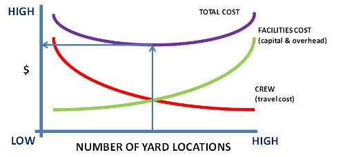
Figure 1

Using all the inputs mentioned previously, a series of calculations is performed to estimate:
• Proximity between staging locations and work sites;
• frequency and duration of maintenance crew visits at each work site;
• travel time between staging locations and work sites;
• annual travel cost summary for each staging location and work site;
• annual building operations and maintenance cost;
• capital cost of constructing new staging locations;
• benefit of removing a yard from service through rent/sale/leasing;
• cost of renovations when consolidating staging locations; and
• total cost of existing compared with each potential configuration.

Proximity is the distance between a staging location and work site. This can be calculated precisely from GIS or other map service data. Trip frequency can be obtained from existing systems or estimated based on other input data. Duration of maintenance effort must also be obtained for each work site. For example, if a site requires 20 hours of maintenance, the average crew size was 2.5, and an average onsite time of 4 hours, then the trip frequency can be calculated as follows:

Trip Frequency = (required labor hours)/(crew size * onsite time)

Trip Frequency = (20)/(2.5 * 4) = 2 trips required per year

Again, some computerized systems can greatly assist in this effort when configured correctly.

Travel time is a function of the proximity, trip frequency, and road speed. First, the one-way travel time is calculated in terms of hours. This is then multiplied by the trip frequency to determine the annual travel time. The formulas for one-way travel time and annual travel time are shown below with examples.

Travel Hours = (Proximity in miles/Travel Distance in mph)

Annual Travel Hours = Travel Hours * Trip Frequency

Travel Hours = (5/35) = 0.14 hour (approximately 8.5 minutes)

Annual Travel Hours = 1/7 * 2 = 0.29 hour (approximately 17.1 minutes)

Resource values are used to determine the cost of travel and include labor, overhead, and equipment costs. An example formula is shown below using an estimated labor rate of $25 per hour, overhead of 130 percent, a crew size of 2.5, and an hourly equipment rate of $15.

Annual Travel Cost = (Annual Travel Hours) * (((labor rate * (1 + overhead)) * crew size) + equipment rate)

Annual Travel Cost = 0.29 * (((25 * (1+130%)) * 2.5) + 15) = $45.36 annual travel cost to site

The following real estate and capital costs must also be collected or estimated:
• building operations and maintenance;
• new construction; and
• rental/leasing/renovations.

Operations and maintenance costs would apply to all work staging locations. This includes proposed locations that may not yet exist. New construction costs would apply when a new yard is being proposed, while rental/leasing/renovation costs would apply when yards are being removed from service and resources consolidated at existing facilities. These values should be annualized over the estimated useful life of the staging location.

The total cost for a configuration is determined by adding together all travel, operations, capital, and any renovation costs. The total cost is offset by any rental benefits or reductions in travel cost. Comparing these total cost summaries for each potential configuration to the existing configuration will identify any substantial differences in cost and determine the magnitude of the impact when related to each other. An example of this summary and comparison for Santa Clara is shown in Figure 2.

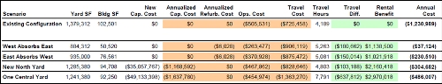
Figure 2

Other practical applications

Analysis of maintenance yard staging locations can be useful for many applications. The need to analyze any potential impact of downsizing or constructing new staging locations is critical when planning for development or restructuring an organization or service area. As discussed in the case studies, a formulated approach can be used to optimize staging locations, resulting in reduced travel time and related costs. The case studies also demonstrate the ability to estimate staffing and equipment needs by projecting workload with the ability to adjust variables.

Summary

Yard locations with staged resources fundamentally define your operations and determine all operational costs associated with work activities. As a result, it may be an opportunity to re-visit existing yard locations to determine if an MSLM can provide a viable alternative yard configuration for your city or county. The bottom line is increased operational efficiencies and significant annual savings that ultimately help improve resource allocation for public infrastructure.

Gene Hewitt is manager of administrative services, Road Maintenance Division, Roads and Airports Department, Santa Clara County. He can be contacted at gene.hewitt@rda.sccgov.org. Amie Drotning is senior associate with LA Consulting and a member of the American Public Works Association's Southern California Chapter. She can be contacted at adrotning@laconsulting.com. Hewitt and Drotning presented on this topic at the 2012 Public Works Congress and Expo in Anaheim, Calif.

Return to: 2012 Feature Stories